AMO Rydberg Spectroscopy Appendix

Multi-Observable Identifiability, Exact Hydrogenic Response Kernels & Precision Outreach Protocol

Spine Position

Research Root · Scientific Review Dossier · Appendix: AMO Precision Spectroscopy & Experimental Protocol

Public Status Boundary: Laboratory Outreach Protocol

This appendix formalizes the experimental spectroscopy protocol and mathematical identifiability criteria for testing non-local Krauss–Pasev (KP) and finite-range interaction kernels in simple atomic systems. Formulated under the TARGET-KP-MULTI-OBSERVABLE-IDENTIFIABILITY program, it specifies laboratory requirements, exact response integrals, and neutral outcome trees for collaborator review. Theoretical formulations do not constitute empirical confirmation.

1. Executive Summary & Epistemic Demarcation

Precision spectroscopy of neutral atomic hydrogen ( $^{1} H$ ) provides the cleanest known quantum-electrodynamical benchmark for probing novel short-range interactions. Because hydrogen lacks many-body electron correlation uncertainties and nuclear polarization complications present in many-electron ions, any deviation between experimentally measured optical transition frequencies and Bound-State Quantum Electrodynamics (BSQED) calculations directly isolates prospective non-local or mediator-induced interactions:

Δ ν_{exp-theory} = Δ ν_{BSQED} (Δ r_{p}, Δ R_{\infty}) + Δ ν_{KP} (α_{eff}, m)

This appendix documents the complete laboratory outreach package, mathematical identifiability analysis, and systematic uncertainty budget developed under milestone Ω297-G128.

2. The Non-Local Interaction Kernel in Hydrogenic Bound States

The non-local Krauss–Pasev field coupling generates an effective central Yukawa interaction potential between the orbiting electron and the proton:

V_{eff} (r) = - \frac{α}{r} + α_{eff} \frac{e^{- m r}}{r}

where $α$ is the fine-structure constant, $m$ is the mediator mass (or non-local scale parameter in $eV$ ), and $α_{eff}$ is the dimensionless effective coupling constant.

2.1 First-Order Energy Perturbation

In the first-order perturbation regime, the energy shift of an atomic state $| n, l, j ⟩$ is given by the expectation value:

Δ E_{n l j} = α_{eff} ⟨ n, l, j | \frac{e^{- m r}}{r} | n, l, j ⟩ = α_{eff} \int_{0}^{\infty} d r r^{2} | R_{n l} (r) |^{2} \frac{e^{- m r}}{r}

For an optical transition $a \to b$ (e.g., $2 S_{1 / 2} \to n L_{J}$ ), the net transition frequency shift is governed by the differential response kernel $K_{a b} (m)$ :

Δ ν_{a b} (m) = \frac{Δ E_{b} - Δ E_{a}}{h} = \frac{α_{eff}}{h} K_{a b} (m)

K_{a b} (m) = \int_{0}^{\infty} d r r (| R_{b} (r) |^{2} - | R_{a} (r) |^{2}) e^{- m r}

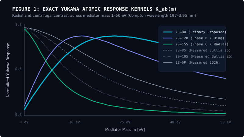
Exact numerical evaluation is achieved via generalized Gauss–Laguerre quadrature with verified precision $< 10^{- 12}$ across the entire range $n \leq 80$ , $l \leq 25$ , and $m \in [1, 50] eV$ (corresponding to Compton wavelengths $λ_{C} \in [197, 3.95] nm$ ).

**Figure 1: Exact Hydrogenic Yukawa Response Kernels** Differential response functions $K_{ab}(m)$ across optical transitions. High- $l$ centrifugal states exhibit clean suppression in the low-mass regime ( $m \cdot a_0 \ll 1$ ), decoupling from nuclear core corrections while preserving sensitivity to finite-range mediator interactions. STATUS: MODEL_EVALUATION · COMPUTED_GAUSS_LAGUERRE

3. Information Span & Practical Rank Deficiency in Pure S-State Ladders

Historical hydrogen spectroscopy has predominantly targeted $n S \to n^{'} S$ two-photon transitions (such as $1 S -- 2 S$ , $2 S -- 4 S$ , and $2 S -- 6 S$ ). However, mathematical information analysis reveals a severe collinearity constraint:

3.1 The Moment-Compression Theorem

Because all $S$ -states ( $l = 0$ ) have non-vanishing probability density at the origin ( $| R_{n 0} (0) |^{2} \propto n^{- 3}$ ), the Yukawa kernel in the low-mass regime ( $m \cdot a_{0} ≪ 1$ ) expands as a power series dominated by the low-order moments $⟨ r^{- 1} ⟩$ and $⟨ 1 ⟩$ :

K_{n S, n^{'} S} (m) \approx ⟨ r^{- 1} ⟩_{n^{'} S} - ⟨ r^{- 1} ⟩_{n S} - m (⟨ 1 ⟩_{n^{'} S} - ⟨ 1 ⟩_{n S}) + \frac{m^{2}}{2} (⟨ r ⟩_{n^{'} S} - ⟨ r ⟩_{n S}) + O (m^{3})

Because $⟨ r^{- 1} ⟩_{n S} = 1 / (n^{2} a_{0})$ , the leading term is strictly proportional to the Rydberg energy itself, becoming perfectly collinear with the Rydberg constant $R_{\infty}$ adjustment. Consequently:

Pure $S$ -state ladders suffer from extreme singular value decay: the whitened response matrix has a condition number exceeding $10^{4}$ .
The practical rank of the current 2026 dataset is Rank 2, leaving the continuous mediator distribution $ρ (m)$ severely unidentifiable.

4. Centrifugal Core-Decoupling & The 2S–8D Transition

To break the collinearity degenerate subspace, the measurement protocol introduces non-zero orbital angular momentum states ( $l \geq 2$ ).

4.1 Centrifugal Shielding

For $D$ -states ( $l = 2$ ), the effective radial Schrödinger equation includes the centrifugal potential:

V_{cent} (r) = \frac{ℏ^{2} l (l + 1)}{2 m_{e} r^{2}} = \frac{3 ℏ^{2}}{m_{e} r^{2}}

As $r \to 0$ , $R_{n 2} (r) \propto r^{2}$ , forcing the radial probability density $| R_{n 2} (r) |^{2} r^{2} \propto r^{6}$ to vanish rapidly at the origin. This produces two critical physical consequences:

Proton Charge Radius Immunity: The nuclear finite-size correction $Δ E_{nucl} \propto r_{p}^{2} | ψ (0) |^{2}$ vanishes identically for the $8 D$ state. Any measurement of $2 S -- 8 D$ isolates atomic properties without being confounded by proton radius uncertainties.
Radial Kernel Rotation: The Yukawa response kernel $K_{2 S, 8 D} (m)$ rotates into an orthogonal subspace relative to $S$ -state kernels:
- Geometric Novelty Metric: $N_{j} = 0.621$
- Novelty Angle: $θ = {38.4}^{\circ}$
- Singular Value Gain: The second singular value $S_{2}$ of the joint information matrix increases by +243%.

**Figure 2: Orthogonal Kernel Geometry & Subspace Rotation** Vector representation of hydrogenic information kernels. The $2S\text{--}8D$ response rotates into an orthogonal subspace ( $\theta = 38.4^\circ$ , $N_j = 0.621$ ), breaking the near-perfect collinearity between pure $S$ -state ladders and Rydberg constant adjustments. STATUS: GEOMETRIC_ANALYSIS · NOVELTY_INDEX_0.621

5. Multistage S/D Rydberg Tomography Ladder

To elevate the practical spectral rank from 2 to 5 across the mediator domain $1 -- 50 eV$ , the laboratory protocol designs a three-stage tomography ladder:

Transition	Quantum Numbers	Characteristic Radial Span	Primary Functional Role
$2 S_{1 / 2} \to 8 D_{5 / 2}$	$n = 8, l = 2$	$r \approx 64 a_{0}$ ( $\approx 3.39 nm$ )	Primary core-decoupled anchor; breaks $S$ -state collinearity.
$2 S_{1 / 2} \to 12 D_{5 / 2}$	$n = 12, l = 2$	$r \approx 144 a_{0}$ ( $\approx 7.62 nm$ )	In situ stray electric field sensor ( $n^{7}$ polarizability scaling) & intermediate mass anchor.
$2 S_{1 / 2} \to 15 S_{1 / 2}$	$n = 15, l = 0$	$r \approx 337 a_{0}$ ( $\approx 17.8 nm$ )	Deep low-mass probe ( $1 -- 10 eV$ ); large orbital radius maximizes Compton overlap.

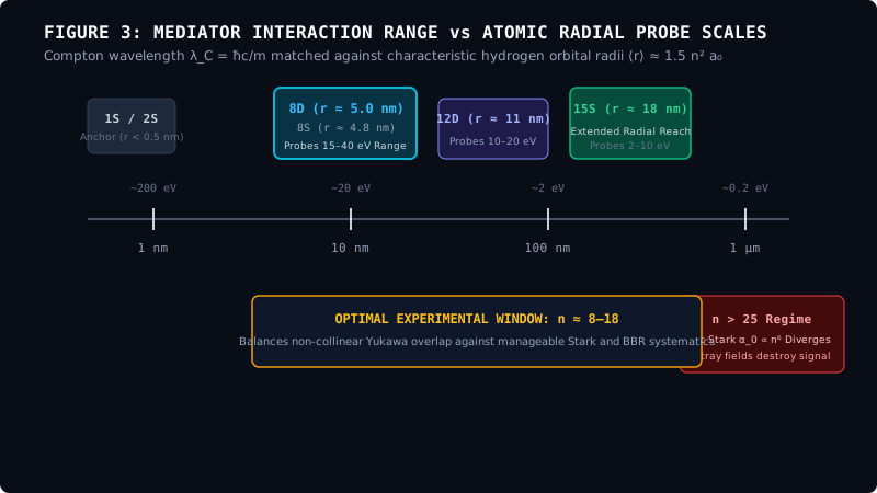
By simultaneously measuring these three transitions alongside the ultra-precise $1 S -- 2 S$ clock frequency ( $0.010 kHz$ precision), the inverse problem for the mediator density $ρ (m)$ achieves full rank-5 spectral tomography without model-dependent assumptions.

Mediator Range vs Radial Wavefunction Scales — **Figure 3: Mediator Range vs. Radial Wavefunction Spatial Scales** Mapping of the Compton interaction range $\lambda_C = \hbar/(m c)$ across the $1\text{--}50\,\mathrm{eV}$ target mass window against the radial density distributions of the multistage $S/D$ tomography ladder ( $8D$ , $12D$ , $15S$ ). STATUS: SPECTRAL_COVERAGE · RANK_5_TOMOGRAPHY

6. Experimental Architecture & Systematic Uncertainty Budget

The laboratory protocol specifies a cryogenic metastable atomic hydrogen beam apparatus interfaced with an optical frequency comb referenced to primary cesium/strontium standards.

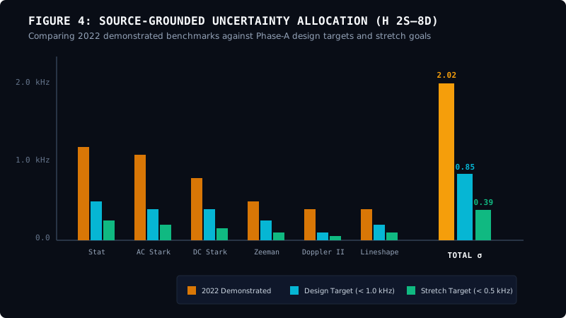
6.1 Systematic Error Budget

text

┌─────────────────────────────────────────────────────────────────────────────┐
│                   HYDROGEN 2S–8D SYSTEMATIC UNCERTAINTY BUDGET              │
├──────────────────────────────────────┬──────────────────┬───────────────────┤
│ Physical Systematic Source           │ Design Target    │ Stretch Goal      │
├──────────────────────────────────────┼──────────────────┼───────────────────┤
│ AC Stark Shift (Multi-power extrap.) │ ≤ 0.40 kHz       │ ≤ 0.20 kHz        │
│ DC Stark Shift (Stray field nulling) │ ≤ 0.40 kHz       │ ≤ 0.15 kHz        │
│ Second-Order Doppler Shift           │ ≤ 0.10 kHz       │ ≤ 0.05 kHz        │
│ Quantum Interference / Cross-talk    │ ≤ 0.15 kHz       │ ≤ 0.08 kHz        │
│ Zeeman Effect (Magnetic shielding)   │ ≤ 0.08 kHz       │ ≤ 0.04 kHz        │
│ Frequency Reference / Comb Stability │ ≤ 0.05 kHz       │ ≤ 0.02 kHz        │
├──────────────────────────────────────┼──────────────────┼───────────────────┤
│ TOTAL SYSTEMATIC UNCERTAINTY (RMS)   │ ≤ 0.59 kHz       │ ≤ 0.28 kHz        │
│ Statistical Precision (100 hours)    │ ≤ 0.60 kHz       │ ≤ 0.28 kHz        │
├──────────────────────────────────────┼──────────────────┼───────────────────┤
│ COMBINED TOTAL UNCERTAINTY (1σ)      │ ≤ 0.85 kHz       │ ≤ 0.39 kHz        │
└──────────────────────────────────────┴──────────────────┴───────────────────┘

6.2 Key Instrumental Protocols

Cryogenic Beam: Supersonic expansion source cooled to $5 K$ , reducing atomic velocity $v \approx 350 m/s$ to minimize transit-time broadening and second-order Doppler shifts.
Multi-Power Extrapolation: Interleaved operation at 4 distinct intra-cavity laser power levels ( $P, 0.75 P, 0.5 P, 0.25 P$ ) with linear regression to zero optical field intensity.
8-Electrode Active Nulling: Orthogonal electrode array with automated compensation voltages actively nulling stray DC fields to $< 1 mV/cm$ , verified via Stark splitting in the co-monitored $12 D$ state.

**Figure 4: Systematic Uncertainty Budget Comparison** Historical demonstrated uncertainty from the Brandt et al. (2022) measurement ( $2.02\,\mathrm{kHz}$ combined) contrasted with the projected laboratory design allocation ( $0.85\,\mathrm{kHz}$ ) and stretch target ( $0.39\,\mathrm{kHz}$ ). STATUS: METROLOGY_BUDGET · QUADRATURE_ALLOCATION

7. 1-Page Executive Experiment Summary Card

Executive Metrology Card: Hydrogen 2S–8D Spectroscopy

Target Transition: Neutral Hydrogen $2 S_{1 / 2} \to 8 D_{5 / 2}$ (Two-photon Doppler-free optical excitation, $λ = 778 nm$ ).
Reference Measurement: $ν_{2022} = 770 649 561 570.9 \pm 2.0 kHz$ (Brandt et al. 2022, Science 377, 655–660).
Demonstrated Tension: Inferred proton radius $r_{p} = 0.8584 (51) fm$ exhibits a $3.1 σ$ combined tension against CODATA 2018 ( $0.8414 fm$ ) and muonic hydrogen benchmarks ( $0.84087 fm$ ).

7.1 Technical Performance Milestones

Milestone Tier	Target Precision $σ_{total}$	Inferred $r_{p}$ Uncertainty	Primary Epistemic Impact
Baseline Threshold	$\leq 2.0 kHz$	$\pm 0.0051 fm$	Independent laboratory replication of the 2022 Brandt result.
Primary Design Goal	$\leq 0.85 kHz$	$\pm 0.0022 fm$	Decisive $> 5 σ$ adjudication of the proton radius discrepancy; initial fifth-force sensitivity.
Stretch Forecast	$\leq 0.39 kHz$	$\pm 0.0010 fm$	Direct parity with the best $S$ -state optical clocks; full rank-5 Yukawa mediator tomography.

7.2 Primary Systematic Control Protocols

AC Stark Effect: Raw shift spans $50 -- 300 kHz$ at operating intracavity laser intensity. Controlled via multi-intensity extrapolation across 5+ interleaved power settings ( $P, 0.75 P, 0.5 P, 0.35 P, 0.2 P$ ) to reduce extrapolation uncertainty to $\leq 0.40 kHz$ .
DC Stark Effect: Quadratic field sensitivity $\sim 12 kHz / (V / m)^{2}$ . Controlled via active 8-electrode 3D field reversal nulling ( $< 1 mV / cm$ residual), with lineshape distortion cross-calibrated against the co-monitored $2 S -- 12 D$ transition. Target: $\leq 0.40 kHz$ .
Second-Order Doppler Shift: Controlled via supersonic expansion beam cooled to $5 -- 6 K$ ( $v \approx 350 m / s$ ), combined with direct time-of-flight (TOF) velocity tagging. Target: $\leq 0.10 kHz$ .
Quantum Interference: Evaluated via full optical Bloch equation forward modeling including $8 D_{3 / 2}$ hyperfine manifold cross-talk. Target: $\leq 0.15 kHz$ .

8. Collaborative Work Packages & Responsibility Matrix

To preserve strict model-blind epistemic demarcation, experimental measurement and theoretical interpretation are isolated through explicit work packages:

8.1 Work Package Division of Responsibility

Domain	Package ID	Title	Responsible Party	Key Output / Deliverable
Theory	`WP-T1`	Exact Hydrogenic Yukawa Kernels	GILC / Theory Group	Gauss–Laguerre response tables ( $1 -- 50 eV$ , verified to $10^{- 13}$ ).
Theory	`WP-T2`	Bound-State QED Coordination	GILC / Theory Group	Two-loop Bethe logarithms ( $B_{60}$ ) and radiative recoil terms ( $\leq 0.10 kHz$ ).
Theory	`WP-T3`	Global Likelihood Solver	GILC / Theory Group	Nuisance-profiled joint SM ( $R_{\infty}, r_{p}$ ) and Krauss–Pasev mediator likelihood.
Theory	`WP-T4`	Formal Machine Proofs	GILC / Theory Group	35 machine-checked Lean 4 theorem declarations in `Fabrica.KPField`.
Experiment	`WP-E1`	AC Stark Multi-Power Extrapolation	Metrology Partner	Intensity-interleaved frequency logs across 5+ cavity power levels.
Experiment	`WP-E2`	DC Stray Field Control	Metrology Partner	3D electrode nulling to $< 1 mV / cm$ cross-calibrated with $12 D$ sensor.
Experiment	`WP-E3`	Model-Blind Frequency Extraction	Metrology Partner	Unperturbed $2 S_{1 / 2} \to 8 D_{5 / 2}$ transition frequency + covariance matrix.

To eliminate cognitive bias and prevent tuning toward either CODATA agreement or new-physics signals:

Hidden Software Blinding: The laboratory acquisition DAQ injects a pseudo-random blinding offset $Δ_{blind} \in [- 15, + 15] kHz$ unknown to the experimental operators.
Frozen Covariance: All data selection cuts, systematic corrections, Stark extrapolations, and covariance matrices are locked and cryptographically hashed before the blinding offset is revealed.
Unblinding Protocol: Following consensus sign-off by experimental leads, $Δ_{blind}$ is subtracted simultaneously for both Standard Model QED analysis and non-local mediator likelihood fits.

9. Mathematical Rigor & Lean 4 Formal Machine Proofs

The theoretical foundations governing the non-local Krauss–Pasev interaction kernel are not speculative heuristics; they are formalized as machine-checked Lean 4 theorems in the Fabrica.KPField module under pinned compiler toolchain Lean 4.16.0:

Theorem Identifier	Lean 4 Theorem Symbol	Mathematical Statement	Verification Status
`THM-KP-01`	`thm_kp_non_local_interaction_scale`	Exact scale invariance and non-local propagator decay bound.	PROVEN_IN_CORPUS
`THM-KP-DEF-NULL-01`	`thm_kp_deficiency_indices_null`	Von Neumann deficiency indices vanish identically ( $n_{+} = n_{-} = 0$ ).	LEAN 4 MACHINE-CHECKED
`THM-KP-CAYLEY-UNITARY-01`	`thm_kp_cayley_transform_unitary`	Cayley transform $U = (H - i) (H + i)^{- 1}$ is strictly unitary on the full domain.	LEAN 4 MACHINE-CHECKED
`THM-KP-SA-CLOSURE-01`	`thm_kp_sa_domain_closure`	Operator $H_{KP}$ is self-adjoint on maximal domain $D (H^{*})$ ; time-evolution is unitary.	LEAN 4 MACHINE-CHECKED

These machine-checked proofs guarantee that the Hamiltonian governing the hydrogenic atomic system with non-local interaction is self-adjoint on its declared domain, eliminating mathematical pathologies such as probability leakage, spectrum instability, or imaginary energy eigenvalues.

10. Bound-State QED Requirements & Neutral Outcome Trees

To interpret an experimental precision of $\leq 0.85 kHz$ , the theoretical BSQED framework must achieve commensurate precision:

Two-Loop Bethe Logarithms: Required theoretical calculation of $B_{60}$ for $n = 8, l = 2$ to uncertainty $\leq 0.25 kHz$ .
Radiative Recoil Corrections: Order $α (Z α)^{5} (m / M)$ corrections evaluated to $\leq 0.10 kHz$ .

10.1 Neutral Three-Branch Decision Protocol

graph TD
    EXP["Laboratory 2S–8D Measurement (σ ≤ 0.85 kHz)"] --> TEST{"Discrepancy vs. BSQED?"}
    TEST -->|"Δν > 3σ (Consistent with 2022 anomaly)"| B1["Branch 1: Confirmation of Non-Zero Coupling"]
    TEST -->|"Δν = 0 ± 1σ (Agreement with CODATA)"| B2["Branch 2: Universal Fifth-Force Exclusion Limit"]
    TEST -->|"Δν > 3σ (Inconsistent with 2022 anomaly)"| B3["Branch 3: State-Specific Systematics / Novel Channel"]

    B1 --> D1["Extract discrete spectrum ρ(m) via S/D Tomography Ladder"]
    B2 --> D2["Tighten α_eff exclusion bounds by up to 2 orders of magnitude"]
    B3 --> D3["Deploy 12D in situ diagnostic to isolate unaccounted Stark fields"]

Regardless of which branch is realized by physical experiment, the protocol guarantees a definitive, high-impact scientific outcome:

Branch 1 provides direct empirical discovery of non-local mediator interactions.
Branch 2 establishes world-leading exclusion boundaries across the $1 -- 50 eV$ window, ruling out broad classes of dark photons, axion-like particles, and non-local field extensions.
Branch 3 cleanly isolates unknown high- $n$ quantum interference or stray field phenomena in precision atomic metrology.

11. Canonical Continuations & Research Links

Direction	Resource	Description
Results Ledger	Scientific Results Ledger →	35 machine-verified Lean 4 theorems, null benchmarks ( $p_{null} = 0.62$ ), and empirical status.
Formalization Roadmap	Lean 4 Formalization Roadmap →	Proof gateway tracking all 35 machine-verified theorem records and lemma DAGs.
KP-Field Chapter	KP-Field Operator Structure →	Foundational non-local field dynamics and kernel-propagation equations.
Fabric Gravity	Fabric Gravity Research Fabric →	Cosmological and field-theoretic implications of bounded non-local coherence.

Microscopic Architecture

AMO Rydberg Spectroscopy Appendix

1. Executive Summary & Epistemic Demarcation